Lecture Two

Link to lecture 2 slideshow: 2_geography.pdf

Notes:

1. Geographical setting:

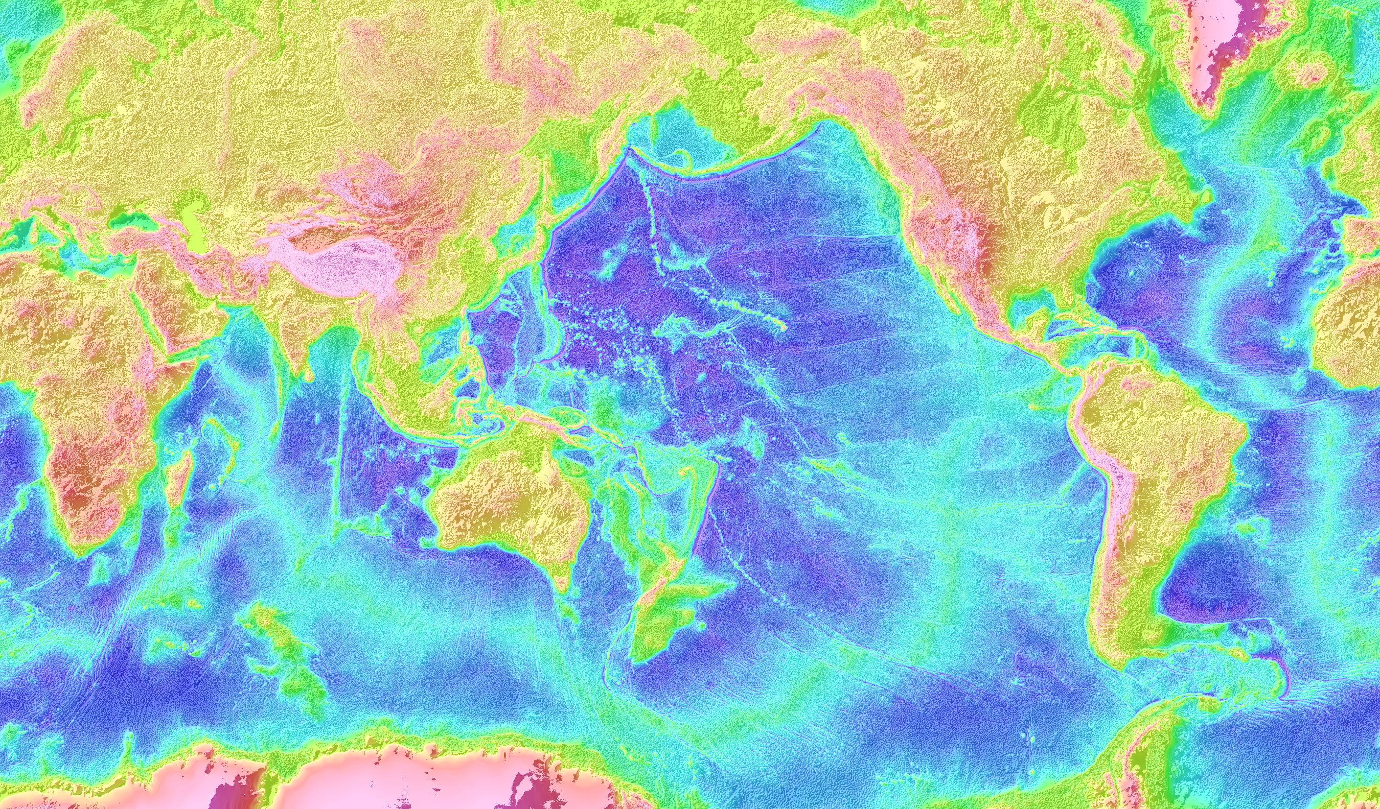
The surface of the Earth consists of continental crust (thick and light) and ocean crust (thin and dense) which “float” on the asthenosphere (1% liquid). The crust (or lithosphere) is separated into several tectonic plates which can move relative to one another. The ocean crust is constantly renewing at the mid-ocean ridges, which are spreading centers (a picture of the seafloor, based on satellite altimetry, can be viewed here).

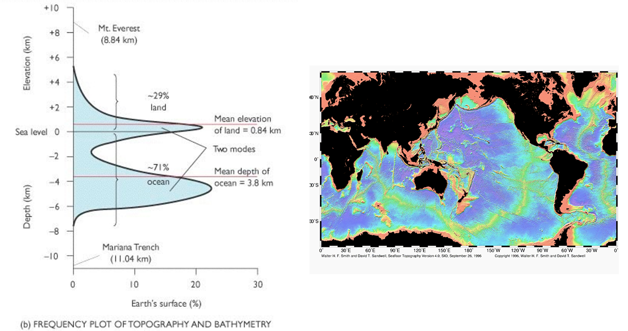
Earth is 70.8% water-covered. In the zonal direction, there is no land between 85-90°N and between 55-60°S. At latitudes 45-70°N there is more land than water. At latitudes 70-90°S there is only land (Antarctica).

The areas of the oceans are: Pacific (179 × 1e6 km²), Atlantic (106 × 1e6 km²), Indian (75 × 1e6 km²). The order of magnitude of the horizontal length scales that we associate with these oceans are: Pacific (15,000 km), Atlantic (5,000 km), Indian (5,000 km).

The Earth's radius (hereafter R_e) is approximately 6371 km. (The Earth is actually not a sphere, but this is close enough for us). The average depth of the ocean is about 4000 m (actually 3795 m). Thus the ocean is a thin skin on the outside of the Earth. The average height of land is 245 m. The maximum elevation is about 9,000 m (Mt. Everest) and the maximum ocean depth is about 11,500 m (Marianas Trench).

1° latitude = (2 pi R_e / 360°) km
1° longitude = (2 pi R_e cos(lat) / 360°) km
1 nautical mile = 1 minute of a great circle of the globe = (2 pi R_e)/(360° × 60) = 1.852 km

• Oceans - Atlantic, Pacific, Indian, Arctic. We often call the region south of about 40°S or 30°S the "Southern Ocean".
• Mediterranean seas - Mediterranean, Arctic, Baltic, Gulf of Mexico, Red Sea, Persian Gulf.
• Marginal seas - many. e.g. Bering Sea, Weddell, South China, Caribbean, Norwegian, Andaman, Arabian.
• Open seas (different properties) - e.g. Sargasso.
• North/South basins - e.g. North Pacific, South Atlantic (because of dynamical divide of equator)

2. Scale analysis:

A very small set of equations governs all the motions of fluids (5 equations for the ocean). This small set governs all scales from nearly-molecular scale to capillary waves to global circulation. As we will see, this set of equations is nonlinear, which means that many terms are products of two things that vary (i.e. velocity times velocity, or velocity times density, etc). We can't possibly solve for all ranges of motion at the same time - direct solutions of the complete governing equations (pencil and paper) are impossible and there simply isn't enough computation power to cover all possible motions. The nonlinearities make theoretical solutions difficult.

Therefore, fluid mechanics is a science of approximation. This differs from the traditional physics and math that you might have studied before, with precise answers and proofs. Advanced applied mathematics includes the rigorous, justified approximation methods used in fluid mechanics. Approximations must be justified. Much of the debate about validity of a particular numerical model of this or that centers on justifying either the physical approximation or the numerical resolution (time and space scales that are resolved). Almost all fluids models include scales of motion that are smaller than the modeled scales. These unresolved processes might impact the outcome of the resolved processes, and so a lot of work goes into "parameterizing" the "sub-grid" scale processes. In theoretical analyses, this step is called "closure".

As a first and necessary step, we evaluate the scales (approximate sizes) of the motion that we wish to resolve. We then perform a rigorous analysis of the governing equations, based on this scale analysis. All properties that characterize the fluid can be scaled - for instance, distance, height, time, velocity (horizontal and vertical), density (variations), temperature, salinity, pressure.

When we want to compare the sizes of two terms that have the same units (i.e. same units in terms of meters, seconds, kilograms, degrees C), we first figure out the approximate sizes (scales) of the terms. The scale of a particular term will have exactly the same units as the term itself. For instance, the time derivative of velocity, du/dt, where u is velocity and t is time, has the scale U/T, where U is the typical size of the velocity, and T is the typical time scale.

Then to compare the two terms, we look at the ratio of the two terms' scalings. In order to compare the two terms, they must have the same units to start with. Therefore the ratio of the two scalings will have no units (units = 1), that is, no length, time, etc. This ratio is called a non-dimensional parameter since it is dimensionless. For example, if we want to compare dw/dt and du/dt, where w is vertical velocity and u is horizontal velocity, the scales of the two terms are W/T and U/T. Each of these dimensional scales has units length/time^2. The non-dimensional ratio of the two is W/U, i.e. no units. If the horizontal and vertical velocities in a particular motion are of about the same size, then this ratio is order (1). If vertical velocity is much smaller than the horizontal velocity, then this ratio is small.

After evaluating the relative size of all of the terms in our equations, using these scalings, which are based entirely on the physical system we are looking at (i.e. is it a surface wave or the whole Pacific general circulation), we then start our modeling. We carefully take into account which terms are small, and ignore them "at first order", meaning in the first step of our analysis. We might look at how they correct the flow later in the same analysis.

A very basic non-dimensional parameter that comes from our discussion of the geographic setting above is the aspect ratio, which is the ratio height/length. For some fluid motions in the ocean, such as surface waves in deep water or convection cells, the aspect ratio is order (1). (That is, the height and length are the same order of magnitude, although they might not be precisely the same number.) In this case, the horizontal and vertical flows for instance could be about the same size. For other oceanic flows, such as surface waves in shallow water or the general circulation, the aspect ratio might be small (order 0.1 or 0.01 or smaller). In this case, motion in the vertical direction will be very different (smaller) than motion in the horizontal direction.

Another very useful ratio is that of the Earth's rotation time scale to the time scale of the motion (~1 day/T). For surface waves, this is a large number, and Earth's rotation is not important. For internal waves, tides, this is order 1, and rotation and changing motion are both important. For the ocean circulation, this ratio is very small, and time dependence is much less important than rotation.

3. Example of scales: the general circulation

• Horizontal spatial scale: 100s to 1000s of kilometers;
• Vertical spatial scale: 1 to 5 km;
• Aspect ratio: H/L = O(.01) to O(.001) << 1;
• Time scales: many years (decades to 100s of years). Small seasonal, interannual to decadal/century changes in flows which basically retain the same patterns as long as the land configuration doesn't change and the atmosphere is dominated by trades and mid-latitude westerlies;
• Earth's rotation time scale relative to time scale of circulation: 1 day/T <<< 1;
• Average current speeds: 1-5 cm/sec (horizontal) in the interior of the ocean, and 50-150 cm/sec (horizontal) in the fastest currents such as the Gulf Stream and Antarctic Circumpolar Current. The vertical velocity for the general circulation is on the order of 10^-4 cm/sec and is almost always inferred, not measured.

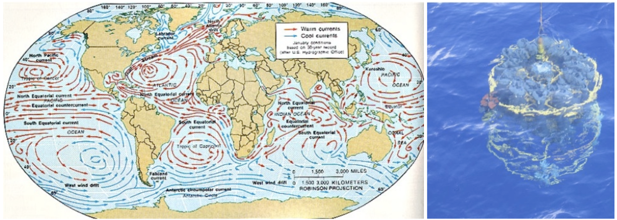
4. Major ocean current system:

• Subtropical gyres - anticyclonic;
• Subpolar gyres - cyclonic;
• Equatorial currents - zonal;
• Western Boundary Currents (fast, deep, warm) - Gulf Stream, Kuroshio, Agulhas Current;
• Eastern Boundary Currents (slow, shallow, cold) - California Current, Peru, Benguela;
• Antarctic Circumpolar Current - only current to circumnavigate globe (no continental boundaries).

• Abyssal circulation (heavily steered by topography);
• Global thermohaline circulation or Meridional Overturning Circulation (in Atlantic).
  

• General introduction and geography: RS 1&2 (skim), 3 (read more carefully)
• Talley et al., Descriptive Physical Oceanography, chapters 1 and 2 (skim), chapter 6.1

Study questions:

1. How much of the Earth is covered with water? In what latitude ranges is the Earth covered by water all the way around? What effect does the presence of continental boundaries at most latitudes have on the circulation? What happens where there is no continental boundary?
2. How deep is the ocean on average? How does this compare with the average zonal dimension of the three major oceans? What effect might this difference between the horizontal and vertical dimensions have on the relative magnitude of the horizontal and vertical velocities? (Another factor affecting the vertical velocities is vertical stratification.
3. What are the forcing mechanisms for the ocean?
4. Check the figure in this link. Assume that the length scale is the "horizontal" length scale (either north-south or east-west) and fill in the approximate length and time scales (order of magnitude) for each of the listed phenomena. You might need to dig through some of the texts on reserve, or search the internet for information, or confer with fellow students. Your answers can be very rough (i.e. mm, cm, m, km, 10s to 100s to 1000s to 10000s km, and similarly rough scales for time).
5. Replace the "time" axis in (4) with a vertical length scale axis. Now place the same phenomena (bubbles to Milankovitch variations) on the new graph, and give the approximate vertical length scales.

Last modified: Aug. 2020